Use of Twenty Years Data of CLUSTER/FGM
to Observe the Mean Behavior of the Magnetic Field
and Current Density of Earth's Magnetosphere

P. Robert^1,2 and M. Dunlop^3,4

¹ Laboratoire de Physique des Plasmas,CNRS, cole polytechnique, Palaiseau, France (retired).
² ScientiDev www.scientidev.fr
³ School of Space and Environment, Beihang University,100191, Beijing, China.
⁴ RAL, Chilton, Oxfordshire, OX11 0QX, UK.

Revision of P. Robert and M. Dunlop , Dec. 2021
Journal of Geophysical Research: Space Physics, 126, e2021JA029837.
https://doi.org/10.1029/2021JA029837>

TECHNICAL REPORTS: DATA
Received 31 JUL 2021
Accepted 9 DEC 2021

CLUSTER FGM: 20 years of data

Idea: use spatial coverage of measurements to get a set of values in a finite volume

- Each point corresponds to a date and a position
- In GSM frame, the hypothesis is made that the mean field depends mainly
  of the dipole tilt angle
- From the measurements we can build grids of field averages values
  which can be used to calculate the intensities and directions of B and J

Cluster 22nd anniversary symposium 7-11 November 2022 / slide

2

In the GSM system we distribute the positions of CLUSTER for 20 years
on a 3D grid of 0.25 RE resolution

Total number of tetrahedron in the cube: ~ 150 10⁶

Cluster 22nd anniversary symposium 7-11 November 2022 / slide

3

- FGM SPIN resolution ( ~ 4s) ; ~ 30 000 CEF files, ~ 45 GB
- binary conversion, with field and position :

FGM_POS_database (~ 30 GB)

- for the calculation of J it is necessary that the 4 measures of B at the vertex
  of the tetrahedron are aligned in time. Same for positions.

Data base creation of FGM_POS_aligned_database

Making 3D grids containing the mean field for various values of θ
(dipole tilt angle). Resolution: 0.25 RE

Cluster 22nd anniversary symposium 7-11 November 2022 / slide

4

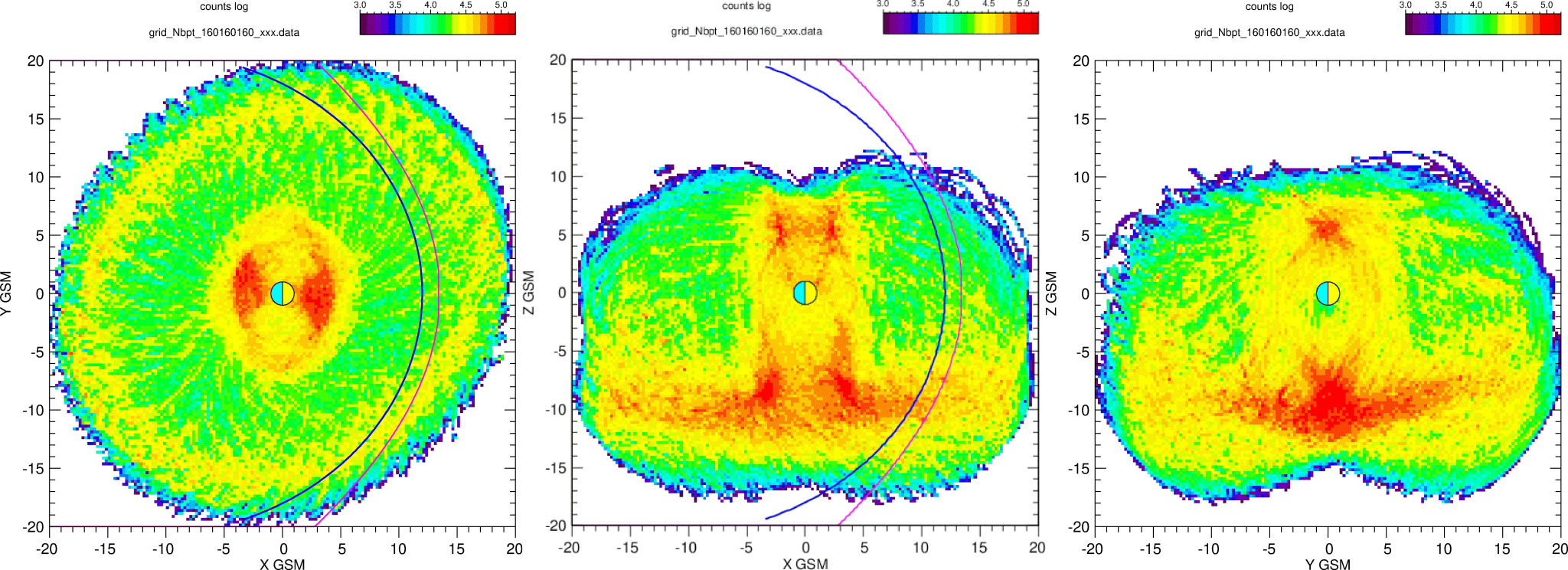
III – OBSERVATION OF
      AVERAGE FIELD

1) Intensity in X-Z GSM
    meridian plane

  => Consistent with
      what is expected

Cluster 22nd anniversary symposium 7-11 November 2022 / slide

5

III – OBSERVATION OF
      AVERAGE FIELD

2) Intensity in X-Y GSM
    equatorial plane

  => Consistent with
      what is expected

Cluster 22nd anniversary symposium 7-11 November 2022 / slide

6

IV - SPATIAL INTERPOLATION

- Grid resolution: 0.25 R_E
- Good compromise between the size of the cells
    and the number of points inside

- Franke–Little interpolation :
    - we collect all the points of the grid inside a sphere of radius R_max
    - each point is at a distance di from the point
      where one wishes the value of the interpolated field
    - each point is assigned a weight W= max(1 – d_i/R_max, 0)
    - and we calculate the average from all the points in the sphere

We can thus have the value of the field at any point
in the 3D space covered by the grid

Note: interpolation from grid: ~ 4 106 points ( [40/0.25]³ )
        interpolation from all initial points : 600 106 points : too heavy for a pc...

Cluster 22nd anniversary symposium 7-11 November 2022 / slide

7

V - B FIELD LINE PLOTS

- as we can have the value of the field at any point in space
   we can calculate field lines with a ray tracing program
   (TRACE de TSY.)


- from a given point, we can calculate the field line starting from this point
   (and in both directions)


- by carefully choosing a set of starting points, one can obtain field lines maps

Cluster 22nd anniversary symposium 7-11 November 2022 / slide

8

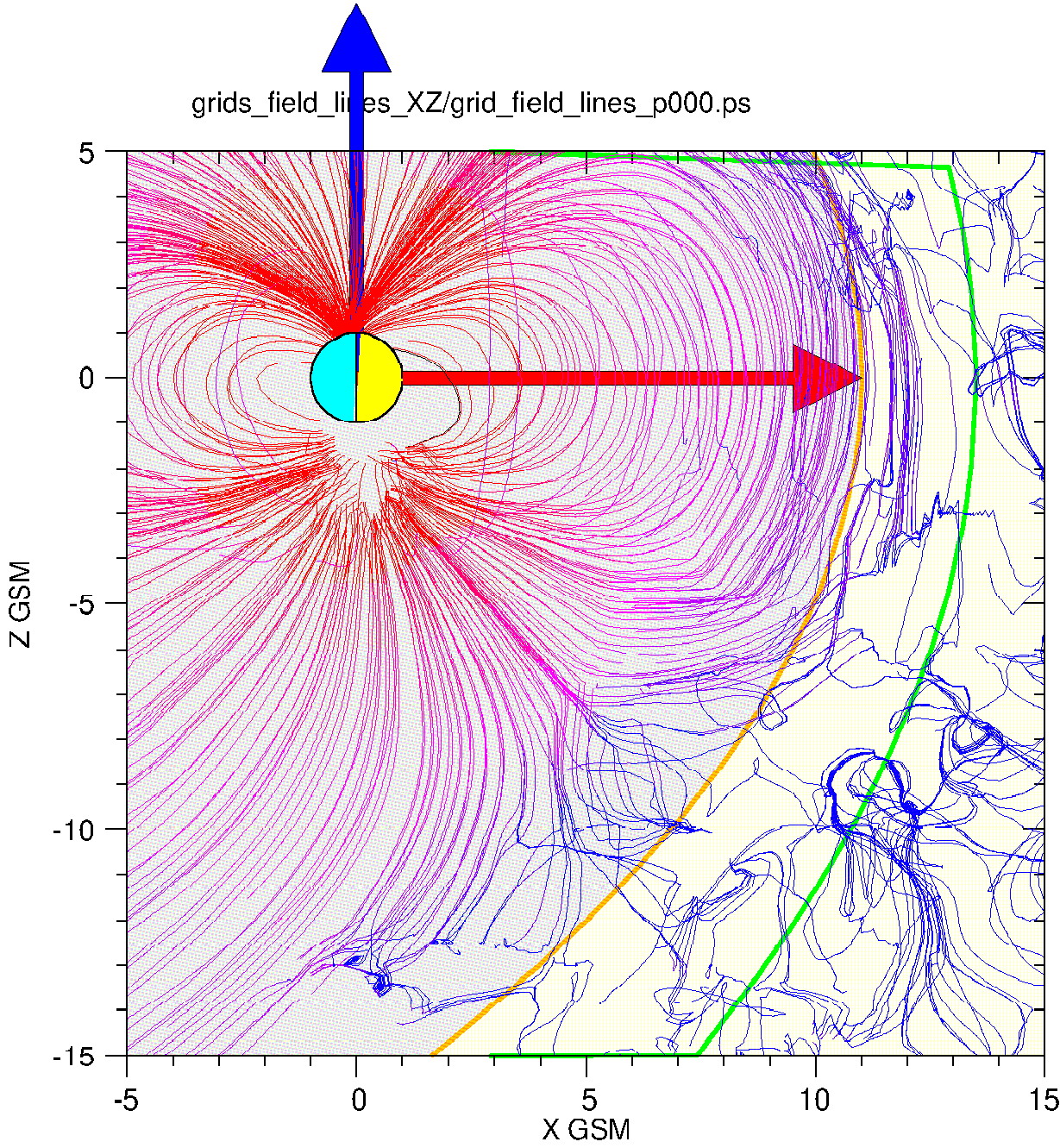
V - B FIELD LINE PLOTS

1) Field lines in X-Z GSM
    meridian plane

  => Consistent with
      what is expected

Cluster 22nd anniversary symposium 7-11 November 2022 / slide

9

V - B FIELD LINE PLOTS

2) Field lines in X-Y GSM
    equatorial plane

  => Consistent with
      what is expected

Cluster 22nd anniversary symposium 7-11 November 2022 / slide

10

V - B FIELD LINE PLOTS

3) Field lines near the Cusps
    (south cusp, θ =0)

very narrow cusp,
with field lines in the center

Cluster 22nd anniversary symposium 7-11 November 2022 / slide

11

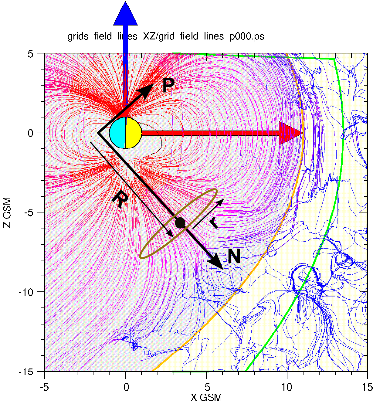
V - B FIELD LINE PLOTS

3) Field lines near the Cusps
    (south cusp, θ =0)

very narrow cusp,
with field lines in the center

→ definition of the NYP system
→ definition of a circular line
    to define the starting point
    (Position R, radius r)

    NYP system

Cluster 22nd anniversary symposium 7-11 November 2022 / slide

12

V - B FIELD LINE PLOTS

4) Field lines of south cusp
    according r (θ =0, R=6)

for r < 0.7 → regular lines
beyond → escaping lines
                across M.P.

Cluster 22nd anniversary symposium 7-11 November 2022 / slide

13

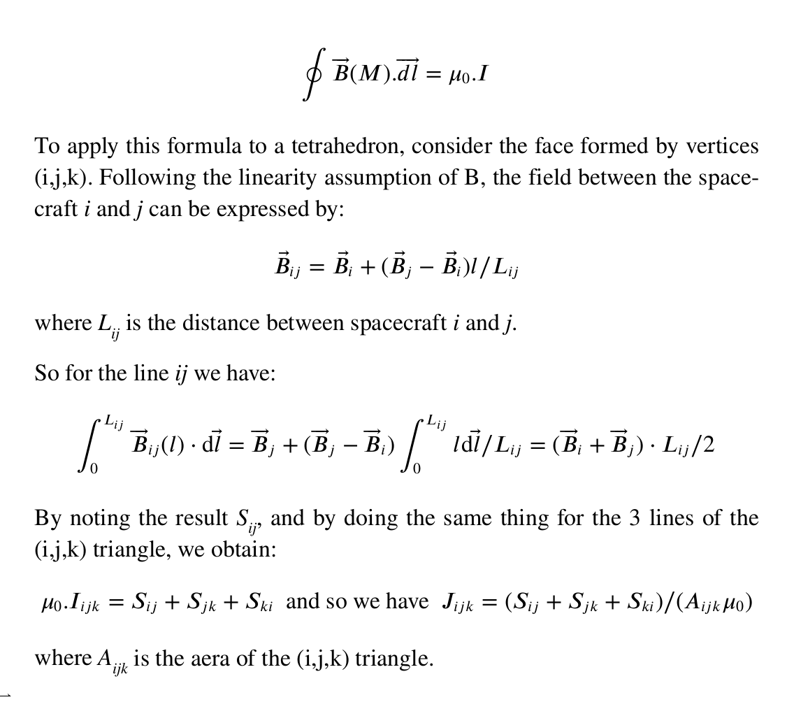
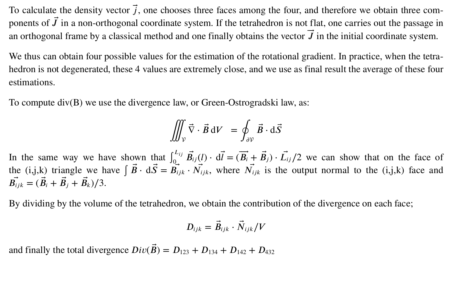
VI - CURL(B) and DIV(B)

1) Computation reminder

Cluster 22nd anniversary symposium 7-11 November 2022 / slide

14

VI - CURL(B) and DIV(B)

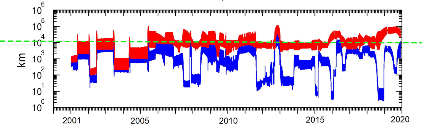
2) Checking method

- removing degenerated tetrahedron (E, P > 0.9)
- limited tetrahedron size: D_max = 10 000 km
- removing IGRF field from B before computation

Cluster 22nd anniversary symposium 7-11 November 2022 / slide

15

VI - CURL(B) and DIV(B)

3) Two ways to compute J

1 - Take all experimental tetrahedra

→ use FGM_POS_aligned_database

2 - Take B values inside the 3D grid of B_ave
    and define a virtual tetrahedron by:

→ use FGM_POS_database

Benefit:

- Orthogonal tetrahedron:
- small size tetrahedron (0.25 R_E)
- more large data base (does not requires 4 S/C group)

Cluster 22nd anniversary symposium 7-11 November 2022 / slide

16

VI - CURL(B) and DIV(B)

4) Results for method # 1

Jo (nA/m²)      ►

- ring current visible,
- intensity ≈ 5-20 nA/m²
- position aroud 3-8 R_E
- Div/Curl≈ 0.1 - 0.2

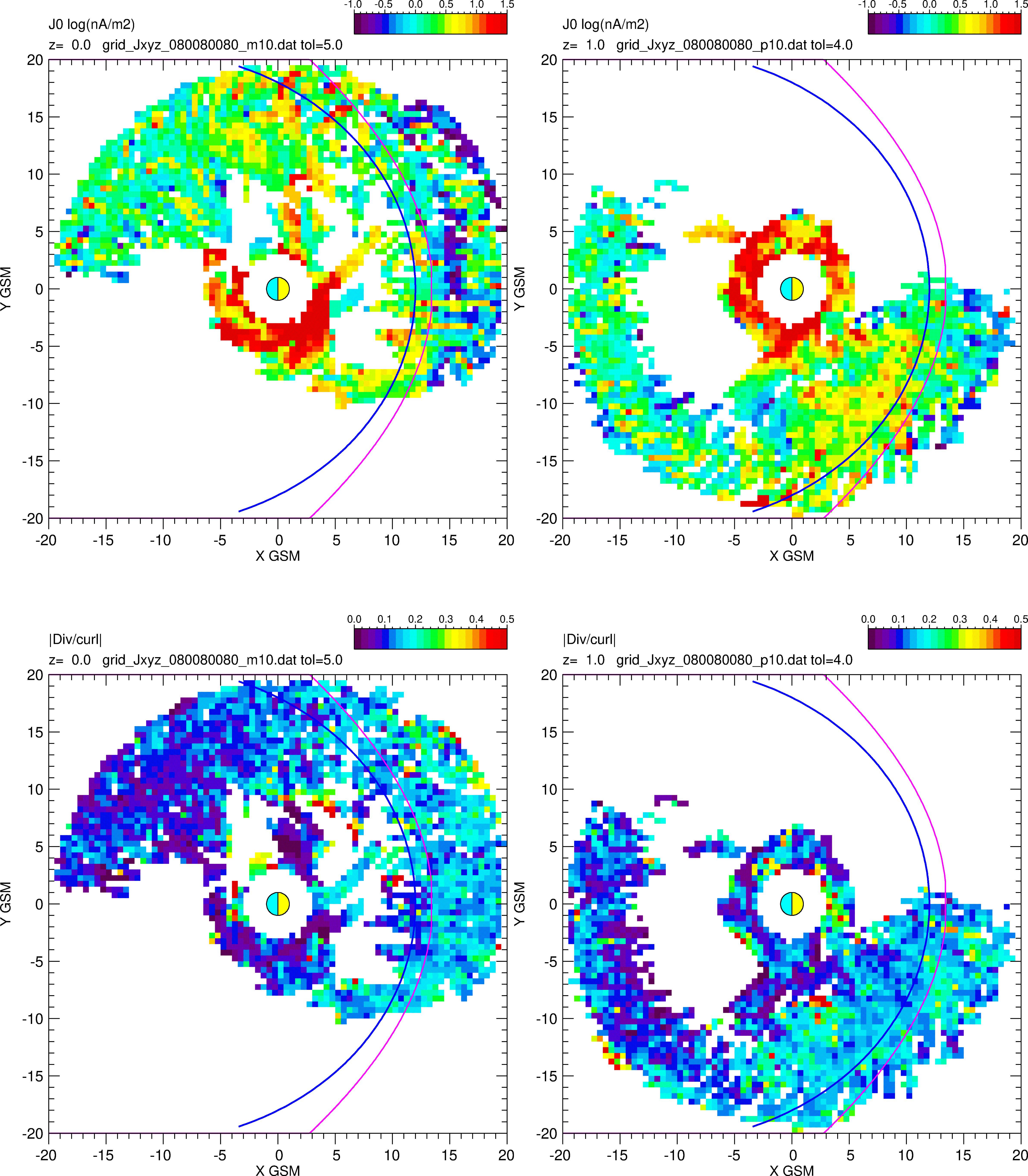
Div/Curl       ►

Cluster 22nd anniversary symposium 7-11 November 2022 / slide

17

VI - CURL(B) and DIV(B)

4) Results for method # 2

Jo (nA/m²)      ►

- better defined ring current,
- same intensity, ≈ 5-20 nA/m²
- same position aroud 3-8 R_E
- Div/Curl≈ 0.1 - 0.2

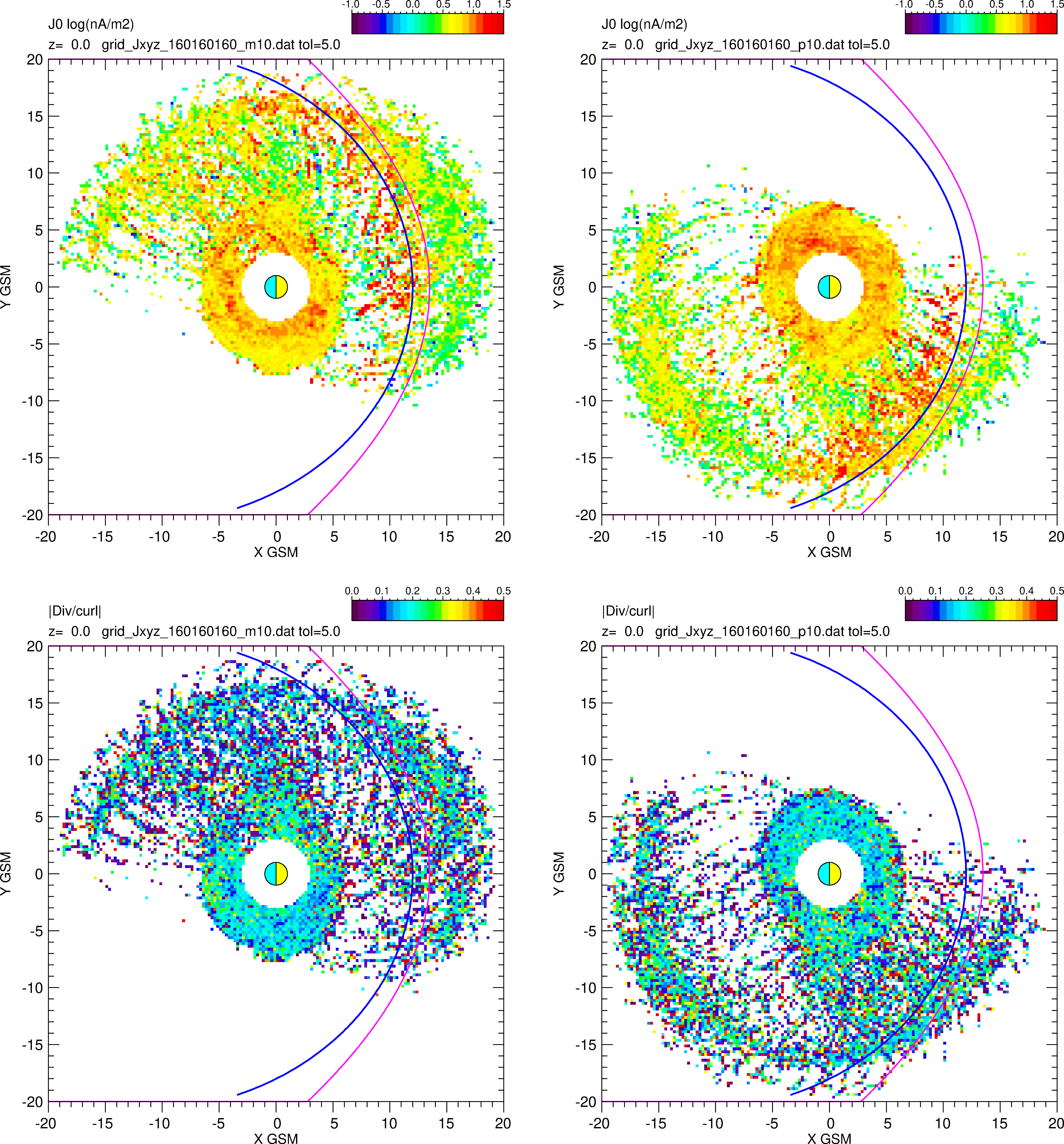
Div/Curl       ►

Cluster 22nd anniversary symposium 7-11 November 2022 / slide

18

VI - CURL(B) and DIV(B)

5)Intensity in X-Z GSM
    meridian plane

well-defined ring current
when coverage is good,
depending on the value of θ

currents near the MP

Cluster 22nd anniversary symposium 7-11 November 2022 / slide

19

VII - J FIELD LINE PLOTS

1)Field line in X-Y SM
    equatorial plane

not so good but R.C.
still visible

Cluster 22nd anniversary symposium 7-11 November 2022 / slide

20

VIII - CUSP MOTION

- B Field line in Y-Z GSE
  for 24 hours
  (the sun is behind us)

- another point of view:
  for 24 hours
  (bottom view)

Daily motion visible

Cluster 22nd anniversary symposium 7-11 November 2022 / slide

21

VII - CONCLUSION

- Data base creation of time aligned B and P over 20 years
- Software to read data base and create 3D grids
    (+ curl(B) and div(B) computation)
- 3D grids creation for B, J, div(B), (J,B) angle etc.
- 3D interpolation to get B(x,y,z,θ)
- possibility of drawing field lines for B and J
- production of B and J maps, in module and in direction
- production of B and J field line maps

→ possibility to add other criteria than θ (solar wind parameters etc.)
→ possibility to add data in addition to CLUSTER (THEMIS, MMS...)

data bases, software and other results available here:   http://roserv.ddns.net/DATA_JGR
JGR paper is available here: http://www.scientidev.fr/FTP_server/Publications/Articles
This talk is available here: http://www.scientidev.fr/FTP_server/Publications/Communications

Cluster 22nd anniversary symposium 7-11 November 2022 / slide

22

HOMAGE

I dedicate this paper to the memory of Alain Roux, with whom I have collaborated all my life.

Alain did the theory and I did the calculations and data processing. We have written many papers together, and this is the first, and probably the last, what I do without him.

Alain would be very happy to see everything we've done with Cluster since his departure, and I pay tribute to him here.

P.R.

Cluster 22nd anniversary symposium 7-11 November 2022 / slide

23